

Modern search and RAG systems are powered by dense retrieval; however, practitioners are confronted with a frustrating tradeoff: bi-encoders are fast but imprecise, while cross-encoders are accurate but too sluggish for production. The operational complexity of dual-model serving is eliminated in this article, and a practical approach is presented that obtains cross-encoder quality from a single bi-encoder through listwise knowledge distillation. This approach also delivers 19% recall improvements over baseline embeddings.
The Tradeoff Between Deployment Simplicity and Retrieval Quality
Typically, production retrieval systems depend on bi-encoders (dual-encoders) to independently embed queries and documents into a shared vector space. This architecture facilitates the precompilation of document embeddings at index time and the execution of a rapid approximate nearest neighbor search at query time. The workhorses of semantic search are models such as BGE, Sentence-BERT, and E5.
The issue is that bi-encoders fail to detect subtle relevance signals. They are unable to simulate the fine-grained interactions between query terms and document content because they encapsulate queries and documents separately. This is resolved by cross-encoders, which jointly process query-document pairs through a single transformer, thereby facilitating comprehensive token-level attention. Cross-encoders consistently outperform bi-encoders on ranking benchmarks, indicating a substantial accuracy gap.
A two-stage pipeline is the conventional approach: first, candidates are retrieved using a bi-encoder, and then they are reranked using a cross-encoder. This is functional; however, it introduces operational burden, infrastructure complexity, and latency. REFINE and other recent methods endeavor to address this lacuna by utilizing model fusion to maintain both a frozen pretrained model and a domain-adapted model with weighted embedding interpolation at inference time. Although effective, this results in a doubling of memory requirements and the introduction of tunable fusion weights that may differ across domains.
The method outlined in this document employs a distinct approach: the ranking knowledge of the cross-encoder is directly transferred to a single bi-encoder through knowledge distillation, and the bi-encoder is subsequently deployed exclusively. No runtime interpolation, no dual-model serving, and no fusion.
Key Concepts: A Concise Overview
The following is a concise explanation of the fundamental concepts before we delve into the method. Readers who are already acquainted with these may proceed to the subsequent section.
Cross-encoder vs. bi-encoder
A bi-encoder generates fixed-size embeddings for queries and documents independently by employing two distinct (often weight-shared) encoders. Relevance is determined by the similarity (usually cosine or dot product) between these embeddings. This independence facilitates precomputation, but it restricts expressiveness.
The query and document are concatenated into a single input sequence by a cross-encoder: [CLS] query [SEP] document [SEP]. The transformer is capable of processing both simultaneously, enabling the full cross-attention of query and document tokens. A relevance score is generated by passing the [CLS] token output through a classification head. This joint processing captures more complex interactions; however, it necessitates evaluating each candidate at query time.
InfoNCE Contrastive Loss
Contrastive learning with InfoNCE loss is the conventional method for training bi-encoders. The model is prompted to attribute a higher similarity to the positive document in the presence of a query, one positive document, and numerous negative documents by the loss.
L_InfoNCE = -log( exp(sim(q, d+) / τ) / Σ exp(sim(q, di) / τ) )
The distribution’s precision is determined by the temperature τ. This loss evaluates relevance as binary: a document is either positive (label=1) or negative (label=0). It is not possible to convey that one negative is “almost relevant” and another is “completely irrelevant.”
Expertise in Soft Labels and Distillation
The transmission of learned behavior from a teacher model to a student model is facilitated by knowledge distillation. The student is taught to replicate the probability distribution of the teacher’s output, rather than being trained on rigid labels (0 or 1). The student learns that A is more relevant than B, despite the fact that both are technically negatives, because these “soft labels” preserve ranking information. For example, if the teacher assigns 40% probability to document A and 10% to document B, the student will learn that A is more relevant.
The extent to which probability mass is distributed among candidates is determined by temperature scaling during softmax generation. Softer distributions are generated by elevated temperatures, which transmit more complex ranking signals.
The Advantages of Listwise Over Pointwise and Pairwise
Each document is evaluated independently using pointwise methods. Document pairs are the focus of pairwise approaches. The ranking of all candidates is directly optimized through listwise approaches, which consider the entire candidate set simultaneously. A single probability distribution encodes the teacher’s full ranking preference across all candidates in listwise soft labels for knowledge distillation, providing a more comprehensive supervision than evaluating documents individually or in pairs.
The Methodology : Listwise Knowledge Distillation
The framework is comprised of two stages: data augmentation through hard negative mining and teacher-student distillation. The complete pipeline is depicted in the diagram below.
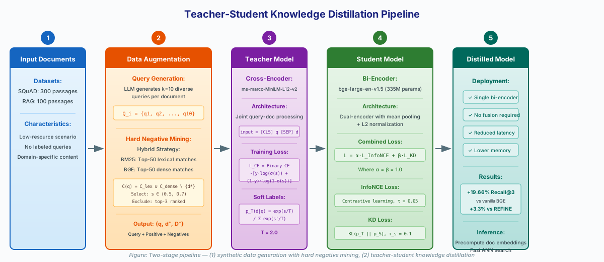
Stage 1: Synthetic Query Generation
In data-scarce circumstances, labeled query-document pairings are unavailable. The initial phase is creating synthetic questions using a large language model. An LLM constructs ten different queries that each document in the corpus could answer. This generates training signals without human annotation.
The prompt directs the LLM to create queries that address several parts of the material, including factual questions, detail-seeking queries, and inference-based questions. Diversity is important since a model trained on the same query types would not generalize successfully..
Stage Two: Hard Negative Mining
Effective contrastive learning necessitates the use of hard negatives: documents that appear to be comparable to the positive but do not answer the question. Easy negatives (random documents) generate a weak training signal because the machine can differentiate them easily.
This approach employs a hybrid strategy that integrates lexical and dense retrieval:
- Retrieve the top 50 documents using BM25 (lexical matching).
- Retrieve the top 50 documents using the vanilla bi-encoder (dense matching).
- Take the union and exclude the ground truth affirmative.
- Filter for papers with similarity scores between [0.5, 0.7].
- Exclude documents that appear in the top three of either retriever.
The filtering guarantees that negatives are problematic (similarity > 0.5), but not too similar to be important (similarity < 0.7). Excluding the top three results avoids false negatives, which occur when the retriever accurately identifies important documents that are not in the ground truth.
Stage 3: Cross-Encoder Teacher Training.
The teacher is a cross-encoder fine-tuned for the synthetic query-document pairings with binary cross-entropy loss.
# Cross-encoder training loss
L_CE = -[y * log(σ(s(q, d))) + (1 - y) * log(1 - σ(s(q, d)))]
Where s(q, d) is the raw relevance score from the cross-encoder, σ is sigmoid, and y ∈ {0, 1} indicates positive or negative pairs.
The base model in this work is cross-encoder/ms-marco-MiniLM-L12-v2, which has been fine-tuned for two epochs with a learning rate of 2e-5 and a batch size of 16. The cross-encoder is small (33 million parameters) yet provides effective ranking supervision.
Stage 4: Soft Label Generation
Once trained, the cross-encoder creates soft labels for the pupil. For each query and its candidate set (positive + negatives), the teacher rates all candidates and transforms scores to a probability distribution using temperature-scaled softmax:
def temperature_softmax(scores: List[float], temperature: float) -> List[float]:
    """Apply temperature-scaled softmax to convert scores to probabilities"""
    scores_array = np.array(scores) / temperature
    exp_scores = np.exp(scores_array - np.max(scores_array))  # numerical stability
    probs = exp_scores / np.sum(exp_scores)
    return probs.tolist()
Temperature T=2.0 generates soft distributions that retain ranking information while not being unduly peaky. Lower temperatures approach hard labels, whereas higher temperatures spread likelihood more evenly.
The teacher then becomes frozen. These soft labels serve as the supervisory signal for student training.
Stage 5: Student Bi-Encoder Training
The student bi-encoder learns from a mixed aim that balances contrastive learning and knowledge distillation.
def compute_loss(query_emb, doc_emb, teacher_probs, tau=0.05, tau_s=0.1, alpha=1.0, beta=1.0):
    """
    Combined InfoNCE + KL divergence loss

    Args:
        query_emb: Query embeddings
        doc_emb: Document embeddings (positive first, then negatives)
        teacher_probs: Soft label distribution from cross-encoder
        tau: Temperature for InfoNCE contrastive loss
        tau_s: Temperature for student softmax in KD loss
        alpha, beta: Loss weights
    """
    # Compute similarities
    sims = torch.matmul(query_emb, doc_emb.t())

    # InfoNCE loss: maximize similarity to positive (index 0)
    logits_nce = sims / tau
    log_probs = F.log_softmax(logits_nce, dim=-1)
    loss_nce = -log_probs[0]  # negative log probability of positive

    # KD loss: match teacher's probability distribution
    student_probs = F.softmax(sims / tau_s, dim=-1)
    loss_kd = F.kl_div(torch.log(student_probs + 1e-8), teacher_probs, reduction='sum')

    # Combined loss
    return alpha * loss_nce + beta * loss_kd
The InfoNCE component guarantees that the model learns fundamental retrieval: prioritize positives over negatives. The KL divergence component conveys sophisticated ranking knowledge: learn the relative order of candidates as determined by the tutor.
Setting α = β = 1.0 ensures equal weight for both objectives. The student temperature (τ_s = 0.1) is lower than the teacher temperature (T = 2.0), allowing for more accurate predictions during inference time.
The base model is bge-large-en-v1.5 (335M parameters), trained over three epochs with a learning rate of 1e-5 and a batch size of sixteen.
Results:
The technique was tested on two datasets that exemplify low-resource scenarios: SQuAD-300 (300 passes) and RAG-100. These imitate true enterprise scenarios in where just a tiny corpus of domain-specific texts is accessible, with no labeled queries.
| Dataset | Model | MAP | NDCG | MRR@3 | Recall@3 |
|---|---|---|---|---|---|
| SQuAD | Vanilla BGE | 0.763 | 0.789 | 0.763 | 0.866 |
| SQuAD | REFINE (fusion) | 0.846 | 0.866 | 0.846 | 0.923 |
| SQuAD | Teacher-Student KD | 0.913 | 0.935 | 0.915 | 0.953 |
| RAG | Vanilla BGE | 0.863 | 0.858 | 0.904 | 0.937 |
| RAG | REFINE (fusion) | 0.881 | 0.867 | 0.919 | 0.940 |
| RAG | Teacher-Student KD | 0.906 | 0.898 | 0.942 | 0.971 |
Key Findings:
- Soft label supervision greatly improves retrieval quality, as demonstrated by a 19.66% Recall@3 improvement over vanilla BGE on SQuAD.
- Outperforms REFINE by 3.3% in RAG despite eliminating runtime fusion overhead. This demonstrates that straight distillation can match or outperform more sophisticated fusion-based techniques.
- Robust cross-domain generalization: When trained on SQuAD and tested on RAG (out-of-domain), the distilled model achieved 0.939 Recall@3, demonstrating strong performance without catastrophic forgetting.
- Simpler deployment: A single bi-encoder eliminates the dual-model architecture required by fusion approaches, resulting in a smaller memory footprint and inference latency.
Practical Implementation Tips
Temperature selection is important. Teacher temperature T=2.0 works well empirically. Lower values (T=1.0) result in distributions that are too peaked to communicate ranking nuance, but higher values (T=4.0+) spread probability too evenly. To encourage confident predictions, the student’s temperature (τ_s) should be lower than the teacher’s.
Hard negative quality is critical. The [0.5, 0.7] similarity filtering range guarantees that negatives are challenging enough to produce a learning signal but not so similar as to be false negatives. Adjust this range according to your corpus: denser semantic spaces may necessitate narrower ranges.
Teacher quality influences student performance. Prior to creating soft labels, the cross-encoder teacher should obtain excellent accuracy. Ensure that the teacher allocates the highest probability to the positive document for the majority of training examples. If p(positive) < 0.5 frequently, it indicates that the teacher requires additional training or that the data is of poor quality.
Loss weighting can be adjusted. Equal weights (α = β = 1.0) are a suitable default. If the pupil difficulties with fundamental retrieval, increase the α. To emphasize distillation, increase β in coarse ranks.
Computational cost is low. The full pipeline takes about 4 GPU-hours on an NVIDIA A100 (40GB). This is substantially lower than fusion-based techniques, which require several models to be trained and do not incur any inference-time overhead.
When To Use This Approach
This approach is particularly appropriate for:
- Data-scarce domains where labeled query-document pairs are unavailable but unlabeled documents exist.
- Enterprise search over proprietary corpora (internal documentation, legal contracts, medical records).
- RAG applications that need high retrieval quality without reranking latency.
- Resource-constrained deployment where running multiple models is impractical
The strategy may be less appropriate when there is a lot of labeled training data (conventional contrastive fine-tuning may suffice) or when the highest possible accuracy warrants the complexity of reranking pipelines.
Conclusion:
Listwise knowledge distillation provides a realistic way to achieve high-quality dense retrieval without the operational complexities of dual-model serving or runtime fusion. A single bi-encoder can learn relevance signals other than binary positive-negative distinctions by converting nuanced ranking judgments from a cross-encoder into soft probability distributions.
The main takeaway is that ordinary contrastive fine-tuning wastes information. Hard labels ignore the relative ordering of negatives that a cross-encoder naturally produces. Soft labels keep this ranking knowledge, while KL divergence offers a logical method for transferring it.
For practitioners developing retrieval systems in specialized fields, this approach provides an appealing combination of cutting-edge quality, ease of deployment, and low computational requirements. The whole methodology, implementation details, and experimental analysis can be found in the research paper “Distilling Cross-Encoder Signals into Bi-Encoders for Domain Retrieval”.
Author: Suraj Desai