Quantifying Data Drift in Categorical Variables using Characteristic Stability Index (CSI)

Due to the recent advancements in artificial intelligence (AI) and machine learning (ML), organizations are increasing investments in information technology (IT) infrastructure that best supports automation enabled by AI and ML. While these automated systems can guide strategic initiatives of the organization, the performance and reliability of predictions are dictated by the quality of data fed into these automated systems. Any changes in the data characteristics while comparing two separate populations is called data drift. 

Any data drift observed between the current population over which the automated system is predicting compared to the reference population over which the automated system is trained on can significantly impact the overall prediction accuracy of the decisioning systems. Considering the risks of data drift, the monitoring of attributes or key business variables is critical in production environments to ensure stable inputs to data models leveraged by the automated systems. Tracking data drift enables organizations to tailor business strategies, monitor production changes, and respond to defects in real time. As an example, consider a scenario where there is a model which uses the originating channel of the incoming consumer to decide risk. A sudden drift in applications originating from higher risk channels can negatively affect the overall model performance. To counter this, a business may introduce added strategy rules to limit the overall risk or exposure. This article introduces an adaptive and scalable approach to mitigate risks of data drift and automate the process for data drift detection that can be extended to different organizations and domains.

Introducing CSI to Detect Data Drift

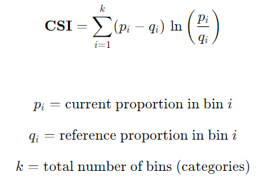
In simple terms, Characteristic Stability Index (CSI) helps quantify the degree of the data drift of categorical variables across any two given populations. The formula to calculate CSI is as follows:

In general, based on the calculated value of CSI, one can evaluate the degree of data drift.

1. If the CSI value is less than 0.1, this signals extremely low drift or no change.
2. If the CSI value is between 0.1 and 0.2, this signals a minor drift.
3. If the CSI value is greater than 0.2, this signals a significant drift.

While these are generalized standard thresholds to measure data drifts, one can change these thresholds depending on business needs. As an example, if an attribute has an exceedingly high importance in the model prediction, the threshold can be lowered to increase the sensitivity of data drift detection. The power of CSI in automating data drift detection in production pipelines lies in its simplicity and standard interpretation that can be easily explained to business users.

Designing Automated Data Drift Frameworks

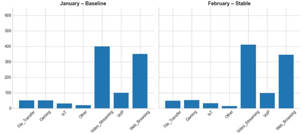
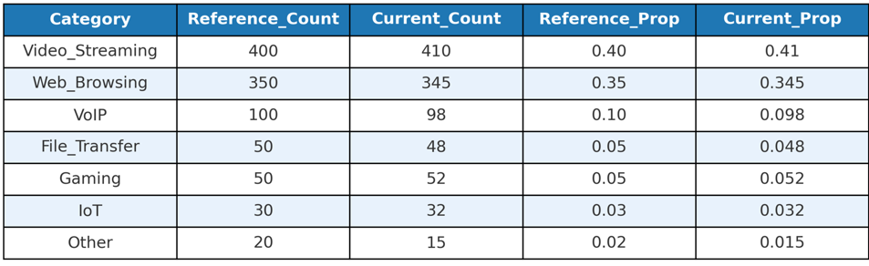
The following section documents the steps involved in developing automated data drift monitoring in production environments. To understand the CSI calculation, we assume a sample attribute called “traffic_type” which tracks the distribution of traffic categories. We capture the data for the traffic_type attribute for the months of January and February. For this analysis, we consider January as the baseline or reference month, while February is considered as the current month. The aggregate volumes for the “traffic_type” for the months of January and February are 1000 rows each. The data distribution of the “traffic_type” for the months of January and February is as follows:

The steps involved in designing automated data drift frameworks leveraging the CSI metric are as follows:

1. Connect to the database hosting the data
2.  Pull in reference and current populations to be tracked
3.  Identify the specific categorical variables to be tracked
4. Employ the CSI calculation
   1. Identify individual categories as bins on the reference population
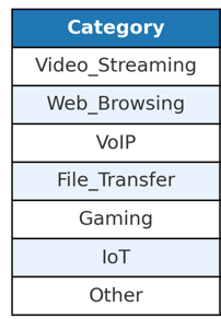
      1. Considering the January month of the attribute “traffic_type”, we list the individual categories such as File_Transfer, Gaming, IoT, Other, Video_Streaming, VoIP and Web_Browsing.

2. Once the bins are identified on the reference population, the same bins are enforced upon the current population to measure distribution of data points.
3. Calculate the reference and current counts for each of the individual categories identified in the previous step.

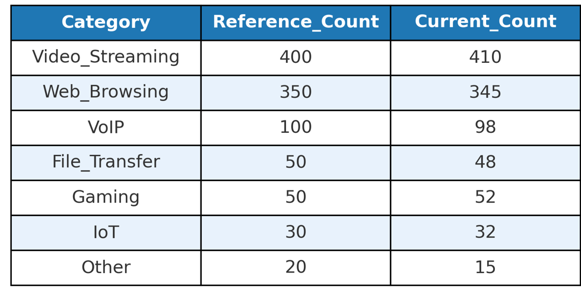
4. Calculate proportions of each individual category for both the reference and current populations. Considering the total aggregate volume for the months of January and February are 1000 each. We divide each category by 1000 to compute their relative proportions.

5.  Using the formula for CSI, we compute CSI contribution values for each of the individual categories.

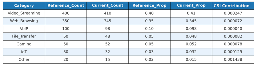
6. Aggregate all the “CSI Contributions” values to compute the final aggregate CSI value for the months of January and February for the attribute “traffic_type”.

5.  Compare the calculated aggregate CSI value against the threshold values for drift sensitivity.
6. Determine if an alert should be triggered or not
   1. If the calculated aggregate CSI value for any of the attributes is greater than the threshold value, then trigger an alert.
   2. If the calculated aggregate CSI value is less than the threshold value, then do not trigger an alert.

These steps described can be executed on a predefined cadence to ensure the automated monitoring runs are executed and teams are aware of any drift that becomes evident in any of the key business variables.

Conclusion

In production systems, data continues to evolve and it is critical for organizations to deploy automated data drift detection frameworks to ensure undetected data drift does not impact downstream analytics or processes. From this demonstration, we were able to validate that CSI offers a practical way to detect distributional changes in categorical attributes to mitigate risks of data drift.  

Author: Anil Cavale